ControlSystemsMTK.jl
ControlSystemsMTK provides an interface between ControlSystems.jl and ModelingToolkit.jl.
See the videos below for examples of using ControlSystems and ModelingToolkit together.
Installation
pkg> add ControlSystemsMTKFrom ControlSystems to ModelingToolkit
Simply calling System(sys) converts a StateSpace object from ControlSystems into the corresponding ModelingToolkitStandardLibrary.Blocks.StateSpace. If sys is a named statespace object, the names of inputs and outputs will be retained in the System as connectors, that is, if my_input is an input variable in the named statespace object, my_input will be a connector of type RealInput in the resulting System. Names of state variables are currently ignored.
Example:
julia> using ControlSystemsMTK, ControlSystemsBase, ModelingToolkit, RobustAndOptimalControl

julia> P0 = tf(1.0, [1, 1])  |> ss
StateSpace{Continuous, Float64}
A =
 -1.0
B =
 1.0
C =
 1.0
D =
 0.0

Continuous-time state-space model

julia> @named P = System(P0)
Model P with 2 equations
States (3):
  x[1](t) [defaults to 0.0]
  input₊u(t) [defaults to 0.0]
  output₊u(t) [defaults to 0.0]
Parameters (0):

julia> equations(P)
2-element Vector{Equation}:
 Differential(t)(x[1](t)) ~ input₊u(t) - x[1](t)
 output₊u(t) ~ x[1](t)
To connect P to the input and output of P, use the connectors P.input and P.output. If the inputs or outputs are multivariable, there are additional scalar connectors for each input/output variable respectively.
Example with named signals
The following creates a named statespace system with named inputs u = :torque and outputs y = [:motor_angle, :load_angle]:
using ControlSystemsMTK, ControlSystemsBase, ModelingToolkit, RobustAndOptimalControl

P = named_ss(DemoSystems.double_mass_model(outputs = [1,3]), u=:torque, y=[:motor_angle, :load_angle])
NamedStateSpace{Continuous, Float64}
A =
0.0 1.0 0.0 0.0
-100.0 -2.0 100.0 1.0
0.0 0.0 0.0 1.0
100.0 1.0 -100.0 -2.0
B =
0.0
1.0
0.0
0.0
C =
1.0 0.0 0.0 0.0
0.0 0.0 1.0 0.0
D =
0.0
0.0
Continuous-time state-space model
With state names: x1 x2 x3 x4
input names: torque
output names: motor_angle load_angle
When we convert this system to a System, we get a system with connectors P.torque and P.motor_angle, in addition to the standard connectors P.input and P.output:
@named P_ode = System(P)\[ \begin{align} \frac{\mathrm{d} x\_{1}\left( t \right)}{\mathrm{d}t} &= x\_{2}\left( t \right) \\ \frac{\mathrm{d} x\_{2}\left( t \right)}{\mathrm{d}t} &= - 100 x\_{1}\left( t \right) - 2 x\_{2}\left( t \right) + 100 x\_{3}\left( t \right) + x\_{4}\left( t \right) + \mathtt{input.u}\left( t \right) \\ \frac{\mathrm{d} x\_{3}\left( t \right)}{\mathrm{d}t} &= x\_{4}\left( t \right) \\ \frac{\mathrm{d} x\_{4}\left( t \right)}{\mathrm{d}t} &= 100 x\_{1}\left( t \right) + x\_{2}\left( t \right) - 100 x\_{3}\left( t \right) - 2 x\_{4}\left( t \right) \\ \mathtt{output.u}\_{1}\left( t \right) &= x\_{1}\left( t \right) \\ \mathtt{output.u}\_{2}\left( t \right) &= x\_{3}\left( t \right) \\ \mathtt{torque.u}\left( t \right) &= \mathtt{input.u}\left( t \right) \\ \mathtt{motor\_angle.u}\left( t \right) &= \mathtt{output.u}\_{1}\left( t \right) \\ \mathtt{load\_angle.u}\left( t \right) &= \mathtt{output.u}\_{2}\left( t \right) \end{align} \]
Here, P.torque is equal to P.input, so you may choose to connect to either of them. However, since the output is multivariable, the connector P.output represents both outputs, while P.motor_angle and P.load_angle represent the individual scalar outputs.
From ModelingToolkit to ControlSystems
A System can be converted to a named statespace object from RobustAndOptimalControl.jl by calling named_ss
named_ss(ode_sys, inputs, outputs; op)this performs a linearization of ode_sys around the operating point op (defaults to the default values of all variables in ode_sys).
Example:
Using P from above:
julia> @unpack input, output = P;

julia> P02_named = named_ss(P, [input.u], [output.u])
NamedStateSpace{Continuous, Float64}
A =
 -1.0
B =
 1.0
C =
 1.0
D =
 0.0

Continuous-time state-space model
With state  names: x[1](t)
     input  names: input₊u(t)
     output names: output₊u(t)

julia> using Plots;

julia> bodeplot(P02_named)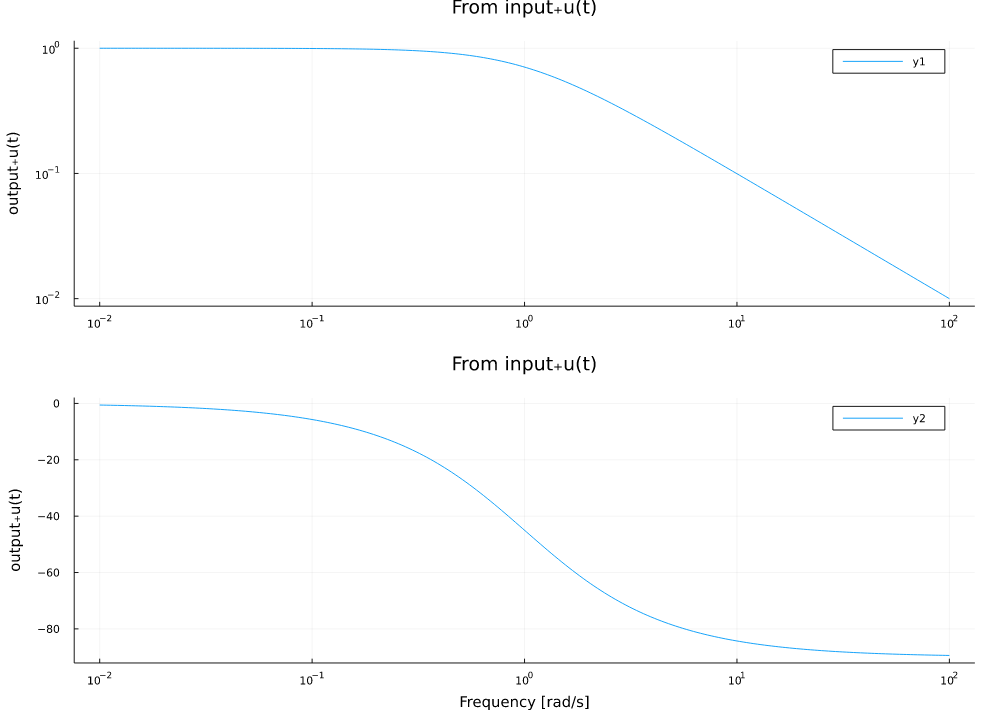
julia> ss(P02_named) # Convert to a statespace system without names
StateSpace{Continuous, Float64}
A =
 -1.0
B =
 1.0
C =
 1.0
D =
 0.0

Continuous-time state-space model
ModelingToolkit tends to give weird names to inputs and outputs etc., to access variables easily, named_ss implements prefix matching, so that you can access the mapping from input₊u(t) to output₊u(t) by
P02_named[:out, :in]To learn more about linearization of ModelingToolkit models, see the video below
Symbolic linearization and code generation
ModelingToolkit has facilities for symbolic linearization that can be used on sufficiently simple systems. The function linearize_symbolic behaves similarly to linearize but returns symbolic matrices A,B,C,D rather than numeric. A StateSpace system with such symbolic coefficients can be used to generate a function that takes parameter values and outputs a statically sized statespace system with numeric matrices. An example follows
System model
We start by building a system mode, we'll use a model of two masses connected by a flexible transmission
using ControlSystemsMTK, ControlSystemsBase
using ModelingToolkit, LinearAlgebra
using ModelingToolkitStandardLibrary.Mechanical.Rotational
using ModelingToolkitStandardLibrary.Blocks: Sine
using ModelingToolkit: connect
import ModelingToolkitStandardLibrary.Blocks
t = Blocks.t

# Parameters
m1 = 1
m2 = 1
k = 1000 # Spring stiffness
c = 10   # Damping coefficient
@named inertia1 = Inertia(; J = m1, w=0)
@named inertia2 = Inertia(; J = m2, w=0)
@named spring = Spring(; c = k)
@named damper = Damper(; d = c)
@named torque = Torque(use_support=false)

function SystemModel(u=nothing; name=:model)
    @named sens = Rotational.AngleSensor()
    eqs = [
        connect(torque.flange, inertia1.flange_a)
        connect(inertia1.flange_b, spring.flange_a, damper.flange_a)
        connect(inertia2.flange_a, spring.flange_b, damper.flange_b)
        connect(inertia2.flange_b, sens.flange)
    ]
    if u !== nothing
        push!(eqs, connect(u.output, :u, torque.tau))
        return @named model = System(eqs, t; systems = [sens, torque, inertia1, inertia2, spring, damper, u])
    end
    System(eqs, t; systems = [sens, torque, inertia1, inertia2, spring, damper], name)
end

model = SystemModel() |> complete
\[ \begin{align} \mathtt{sens.phi.u}\left( t \right) &= \mathtt{sens.flange.phi}\left( t \right) \\ \mathtt{sens.flange.tau}\left( t \right) &= 0 \\ \mathtt{torque.phi\_support}\left( t \right) &= 0 \\ \mathtt{torque.flange.tau}\left( t \right) &= - \mathtt{torque.tau.u}\left( t \right) \\ \mathtt{inertia1.phi}\left( t \right) &= \mathtt{inertia1.flange\_a.phi}\left( t \right) \\ \mathtt{inertia1.phi}\left( t \right) &= \mathtt{inertia1.flange\_b.phi}\left( t \right) \\ \frac{\mathrm{d} \mathtt{inertia1.phi}\left( t \right)}{\mathrm{d}t} &= \mathtt{inertia1.w}\left( t \right) \\ \frac{\mathrm{d} \mathtt{inertia1.w}\left( t \right)}{\mathrm{d}t} &= \mathtt{inertia1.a}\left( t \right) \\ \mathtt{inertia1.J} \mathtt{inertia1.a}\left( t \right) &= \mathtt{inertia1.flange\_a.tau}\left( t \right) + \mathtt{inertia1.flange\_b.tau}\left( t \right) \\ \mathtt{inertia2.phi}\left( t \right) &= \mathtt{inertia2.flange\_a.phi}\left( t \right) \\ \mathtt{inertia2.phi}\left( t \right) &= \mathtt{inertia2.flange\_b.phi}\left( t \right) \\ \frac{\mathrm{d} \mathtt{inertia2.phi}\left( t \right)}{\mathrm{d}t} &= \mathtt{inertia2.w}\left( t \right) \\ \frac{\mathrm{d} \mathtt{inertia2.w}\left( t \right)}{\mathrm{d}t} &= \mathtt{inertia2.a}\left( t \right) \\ \mathtt{inertia2.J} \mathtt{inertia2.a}\left( t \right) &= \mathtt{inertia2.flange\_b.tau}\left( t \right) + \mathtt{inertia2.flange\_a.tau}\left( t \right) \\ \mathtt{spring.phi\_rel}\left( t \right) &= \mathtt{spring.flange\_b.phi}\left( t \right) - \mathtt{spring.flange\_a.phi}\left( t \right) \\ \mathtt{spring.flange\_b.tau}\left( t \right) &= \mathtt{spring.tau}\left( t \right) \\ \mathtt{spring.flange\_a.tau}\left( t \right) &= - \mathtt{spring.tau}\left( t \right) \\ \mathtt{spring.tau}\left( t \right) &= \mathtt{spring.c} \left( - \mathtt{spring.phi\_rel0} + \mathtt{spring.phi\_rel}\left( t \right) \right) \\ \mathtt{damper.phi\_rel}\left( t \right) &= - \mathtt{damper.flange\_a.phi}\left( t \right) + \mathtt{damper.flange\_b.phi}\left( t \right) \\ \frac{\mathrm{d} \mathtt{damper.phi\_rel}\left( t \right)}{\mathrm{d}t} &= \mathtt{damper.w\_rel}\left( t \right) \\ \frac{\mathrm{d} \mathtt{damper.w\_rel}\left( t \right)}{\mathrm{d}t} &= \mathtt{damper.a\_rel}\left( t \right) \\ \mathtt{damper.flange\_b.tau}\left( t \right) &= \mathtt{damper.tau}\left( t \right) \\ \mathtt{damper.flange\_a.tau}\left( t \right) &= - \mathtt{damper.tau}\left( t \right) \\ \mathtt{damper.tau}\left( t \right) &= \mathtt{damper.d} \mathtt{damper.w\_rel}\left( t \right) \\ \mathtt{torque.flange.phi}\left( t \right) &= \mathtt{inertia1.flange\_a.phi}\left( t \right) \\ 0 &= \mathtt{torque.flange.tau}\left( t \right) + \mathtt{inertia1.flange\_a.tau}\left( t \right) \\ \mathtt{inertia1.flange\_b.phi}\left( t \right) &= \mathtt{spring.flange\_a.phi}\left( t \right) \\ \mathtt{inertia1.flange\_b.phi}\left( t \right) &= \mathtt{damper.flange\_a.phi}\left( t \right) \\ 0 &= \mathtt{damper.flange\_a.tau}\left( t \right) + \mathtt{spring.flange\_a.tau}\left( t \right) + \mathtt{inertia1.flange\_b.tau}\left( t \right) \\ \mathtt{inertia2.flange\_a.phi}\left( t \right) &= \mathtt{spring.flange\_b.phi}\left( t \right) \\ \mathtt{inertia2.flange\_a.phi}\left( t \right) &= \mathtt{damper.flange\_b.phi}\left( t \right) \\ 0 &= \mathtt{damper.flange\_b.tau}\left( t \right) + \mathtt{spring.flange\_b.tau}\left( t \right) + \mathtt{inertia2.flange\_a.tau}\left( t \right) \\ \mathtt{inertia2.flange\_b.phi}\left( t \right) &= \mathtt{sens.flange.phi}\left( t \right) \\ 0 &= \mathtt{inertia2.flange\_b.tau}\left( t \right) + \mathtt{sens.flange.tau}\left( t \right) \end{align} \]
Numeric linearization
We can linearize this model numerically using named_ss, this produces a NamedStateSpace{Continuous, Float64}
op = Dict(model.inertia1.flange_b.phi => 0.0, model.torque.tau.u => 0)
lsys = named_ss(model, [model.torque.tau.u], [model.inertia1.phi, model.inertia2.phi]; op)
model: NamedStateSpace{Continuous, Float64}
A =
0.0 0.0 1.0 0.0
0.0 0.0 0.0 1.0
-1000.0 1000.0 -10.0 10.0
1000.0 -1000.0 10.0 -10.0
B =
0.0
0.0
0.0
1.0
C =
0.0 1.0 0.0 0.0
1.0 0.0 0.0 0.0
D =
0.0
0.0
Continuous-time state-space model
With state names: inertia2₊phi(t) inertia1₊phi(t) inertia2₊w(t) inertia1₊w(t)
input names: torque₊tau₊u(t)
output names: inertia1₊phi(t) inertia2₊phi(t)
Operating point: x = [0.0, 0.0, 0.0, 0.0], u = [0.0]
Symbolic linearization
If we instead call linearize_symbolic and pass the jacobians into ss, we get a StateSpace{Continuous, Num}
mats, simplified_sys = ModelingToolkit.linearize_symbolic(model, [model.torque.tau.u], [model.inertia1.phi, model.inertia2.phi])
symbolic_sys = ss(mats.A, mats.B, mats.C, mats.D)
StateSpace{Continuous, Num}
A =
0 0 1 0
0 0 0 1
(-spring₊c) / inertia2₊J spring₊c / inertia2₊J (-damper₊d) / inertia2₊J damper₊d / inertia2₊J
spring₊c / inertia1₊J (-spring₊c) / inertia1₊J damper₊d / inertia1₊J (-damper₊d) / inertia1₊J
B =
0
0
0
1 / inertia1₊J
C =
0 1 0 0
1 0 0 0
D =
0
0
Continuous-time state-space modelCode generation
That's pretty cool, but even nicer is to generate some code for this symbolic system. Below, we use build_function to generate a function that takes a numeric vector x representing the values of the state, and a vector of parameters, and returns a StaticStateSpace{Continuous, Float64}. We pass the keyword argument force_SA=true to build_function to get an allocation-free function.
defs = ModelingToolkit.defaults(simplified_sys)
defs = merge(Dict(unknowns(model) .=> 0), defs)
x = ModelingToolkit.get_u0(simplified_sys, defs) # Extract the default state and parameter values
pars = ModelingToolkit.get_p(simplified_sys, defs, split=false)

fun = Symbolics.build_function(symbolic_sys, unknowns(simplified_sys), ModelingToolkit.parameters(simplified_sys);
    expression = Val{false}, # Generate a compiled function rather than a Julia expression
    force_SA   = true,       # Use static arrays instead of regular arrays, for higher performance 🚀
)

static_lsys = fun(x, pars) # We now have a function that takes state and parameters and returns the linearized system!
StaticStateSpace{Continuous, 2, 1, 4, StaticArraysCore.SMatrix{4, 4, Float64, 16}, StaticArraysCore.SMatrix{4, 1, Float64, 4}, StaticArraysCore.SMatrix{2, 4, Int64, 8}, StaticArraysCore.SMatrix{2, 1, Int64, 2}}
A =
0.0 0.0 1.0 0.0
0.0 0.0 0.0 1.0
-1000.0 1000.0 -10.0 10.0
1000.0 -1000.0 10.0 -10.0
B =
0.0
0.0
0.0
1.0
C =
0 1 0 0
1 0 0 0
D =
0
0
Continuous-time state-space modelIt's pretty fast
using BenchmarkTools
@btime $fun($x, $pars)
8.484 ns (0 allocations: 0 bytes)
faster than multiplying two integers in python.
C-code generation
If you prefer to get C-code for deployment onto an embedded target, the types from Symbolics can be converted to SymPy symbols using symbolics_to_sympy. After this, the function SymbolicControlSystems.ccode is called to generate the C-code. The symbols that are present in the system will be considered input arguments in the generated code.
using SymbolicControlSystems
Asp = SymbolicControlSystems.Sym.(Symbolics.symbolics_to_sympy.(mats.A))
Bsp = SymbolicControlSystems.Sym.(Symbolics.symbolics_to_sympy.(mats.B))
Csp = SymbolicControlSystems.Sym.(Symbolics.symbolics_to_sympy.(mats.C))
Dsp = SymbolicControlSystems.Sym.(Symbolics.symbolics_to_sympy.(mats.D))
sys_sp = ss(Asp, Bsp, Csp, Dsp)

discrete_sys_sp = c2d(sys_sp, 0.01, :tustin) # We can only generate C-code for discrete systems

code = SymbolicControlSystems.ccode(discrete_sys_sp; function_name="perfectly_grilled_hotdogs")
This produces the following code,
#include <stdio.h>
#include <math.h>

void perfectly_grilled_hotdogs(double *y, double u, double damper_d, double inertia1_J, double inertia2_J, double spring_c) {
    static double x[4] = {0};  // Current state
    double xp[4] = {0};        // Next state
    int i;

    // Common sub expressions. These are all called xi, but are unrelated to the state x
    double x0 = inertia2_J*spring_c;
    double x1 = 2.0*x0;
    double x2 = 200.0*damper_d;
    double x3 = inertia2_J*x2;
    double x4 = x0 + x3;
    double x5 = 40000.0*inertia2_J;
    double x6 = inertia1_J*x5;
    double x7 = inertia1_J*spring_c;
    double x8 = inertia1_J*x2;
    double x9 = x7 + x8;
    double x10 = x6 + x9;
    double x11 = 1.0/(x10 + x4);
    double x12 = x11*x[2];
    double x13 = damper_d*inertia1_J;
    double x14 = inertia1_J*inertia2_J;
    double x15 = 1.0/(damper_d*x5 + 200.0*x0 + 40000.0*x13 + 8000000.0*x14 + 200.0*x7);
    double x16 = spring_c + x2;
    double x17 = 0.01*u;
    double x18 = x17*(x16 + x5);
    double x19 = 20000.0*damper_d;
    double x20 = 1.0/(inertia1_J*x19 + inertia2_J*x19 + 100.0*x0 + 4000000.0*x14 + 100.0*x7);
    double x21 = x20*x[3];
    double x22 = x20*x[1];
    double x23 = -x0;
    double x24 = x10 + x3;
    double x25 = x11*x[0];
    double x26 = x0*x12;
    double x27 = x11*x[3];
    double x28 = x11*x[1];
    double x29 = 2.0*x7;
    double x30 = x16*x17;
    double x31 = x4 + x6;
    double x32 = -x7;
    double x33 = x31 + x8;
    double x34 = x25*x7;
    double x35 = x15*x[3];
    double x36 = x15*x[1];
    double x37 = 0.005*u*x15/inertia1_J;

    // Advance the state xp = Ax + Bu
    xp[0] = (x1*x12 + x10*x22 + x15*x18 + x21*x4 + x25*(x23 + x24));
    xp[1] = (-400.0*x0*x25 + x11*x18 + 400.0*x26 + x27*(400.0*damper_d*inertia2_J + x1) + x28*(x10 + x23 - x3));
    xp[2] = (x12*(x32 + x33) + x15*x30 + x21*x31 + x22*x9 + x25*x29);
    xp[3] = (x11*x30 - 400.0*x12*x7 + x27*(x31 + x32 - x8) + x28*(400.0*x13 + x29) + 400.0*x34);

    // Accumulate the output y = C*x + D*u
    y[0] = (x10*x36 + x10*x37 + x24*x25 + x26 + x35*x4);
    y[1] = (x12*x33 + x31*x35 + x34 + x36*x9 + x37*x9);

    // Make the predicted state the current state
    for (i=0; i < 4; ++i) {
        x[i] = xp[i];
    }

}
Additional resources
- Modeling for control using ModelingToolkit tutorial
- Linear Analysis tools in ModelingToolkit
- Video demo using ControlSystems and MTK
Internals: Transformation of non-proper models to proper statespace form
For some models, ModelingToolkit will fail to produce a proper statespace model (a non-proper model is differentiating the inputs, i.e., it has a numerator degree higher than the denominator degree if represented as a transfer function) when calling linearize. For such models, given on the form $\dot x = Ax + Bu + \bar B \dot u$ we create the following augmented descriptor model
\[\begin{aligned} sX &= Ax + BU + s\bar B U \\ [X_u &= U]\\ s(X - \bar B X_u) &= AX + BU \\ s \begin{bmatrix}I & -\bar B \\ 0 & 0 \end{bmatrix} &= \begin{bmatrix} A & 0 \\ 0 & -I\end{bmatrix} \begin{bmatrix}X \\ X_u \end{bmatrix} + \begin{bmatrix} B \\ I_u\end{bmatrix} U \\ sE &= A_e x_e + B_e u \end{aligned}\]
where $X_u$ is a new algebraic state variable and $I_u$ is a selector matrix that picks out the differentiated inputs appearing in $\dot u$ (if all inputs appear, $I_u = I$).
This model may be converted to a proper statespace model (if the system is indeed proper) using DescriptorSystems.dss2ss. All of this is handled automatically by named_ss.
Summary: If you get the error message
Input derivatives appeared in expressions (-gz\gu != 0)
Switch from calling linearize to calling named_ss with exactly the same input arguments, and then pass the argument allow_input_derivatives = true to named_ss.