Manual: Nonlinear Design (DAE)

• Manual: Nonlinear Design (DAE)
• • Nonlinear Model (DAE)

Nonlinear Model (DAE)

In this example, the goal is to control the pH of a solution in a continuously stirred tank reactor (CSTR) for neutralization. The manipulated input is the inlet flow rate of a strong base in L/min, while the inlet flow rate of a weak acid, also in L/min, is a measured disturbance:

\[\begin{aligned} \mathbf{u} &= q_{Bin} \\ \mathbf{y} &= \mathrm{pH} \\ \mathbf{d} &= q_{Ain} \end{aligned}\]

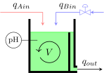
An overflow weir draws the neutralized solution, effectively keeping a constant volume of solution inside the tank. The following figure depicts the pH neutralization process:

Instantaneous Charge Balance

The solution must remain electrically neutral, i.e. the sum of the charges of all ions must equal zero. The ions in this case study are:

• Hydrogen $[\mathrm{H}^+]$
• Sodium $[\mathrm{Na}^+]$
• Hydroxide $[\mathrm{OH}^-]$
• Acetate $[\mathrm{Ac}^-]$

The instantaneous charge balance leads to:

\[0 = [\mathrm{H}^+] + [\mathrm{Na}^+] - [\mathrm{OH}^-] - [\mathrm{Ac}^-]\]

The water dissociation constant and the weak acid equilibrium constant are respectively defined by:

\[\begin{aligned} K_w &= [\mathrm{H}^+][\mathrm{OH}^-] \\ K_a &= \frac{[\mathrm{H}^+][\mathrm{Ac}^-]}{[\mathrm{H}\mathrm{Ac}]} \end{aligned}\]

We respectively denote the algebraic variable and the two states with:

\[\begin{aligned} a_H &= [\mathrm{H}^+] \\ c_A &= [\mathrm{H}\mathrm{Ac}] + [\mathrm{Ac}^-] \\ c_B &= [\mathrm{Na}^+] \end{aligned}\]

in which $c_A$ represents the total concentration of the acid species in the reactor (mol/L), composed of an undissociated acid $\mathrm{H}\mathrm{Ac}$ and the acetate ion $\mathrm{Ac}^-$. Substituting the constants, algebraic and state variables into the charge balance leads the algebraic equation:

\[0 = a_H + c_B - \frac{K_w}{a_H} - \frac{K_a c_A}{K_a + a_H}\]

The pH is computed with:

\[\mathrm{pH} = -10 \log_{10}(a_H)\]

Mass Balance

Applying a mass balance on the weak acid $A$ and the strong base $B$ invariants leads to the differential equations:

\[\begin{aligned} \dot{c}_A(t) &= \frac{60}{V}(q_{Ain} c_{Ain} - q_{out} c_{Aout}) \\ \dot{c}_B(t) &= \frac{60}{V}(q_{Bin} c_{Bin} - q_{out} c_{Bout}) \end{aligned}\]

in which the concentrations $c$ are in mol/L, the tank volume $V$ in L and the volumetric flow rates $q$ in L/min. The accumulation terms $\dot{c}$ are in mol/(L h) because of the 60 factors. By assuming a perfectly mixed reactor and a constant volume because of the weir, the following relations compute the outflow terms:

\[\begin{aligned} c_{Aout} &= c_{A} \\ c_{Bout} &= c_{B} \\ q_{out} &= q_{Ain} + q_{Bin} \end{aligned}\]

The code is:

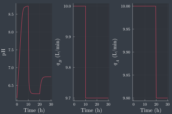
using ModelPredictiveControlV = 1000.0      # reactor volume [L]c_Ain = 0.1     # feed concentration of weak acid [mol/L]c_Bin = 0.1     # feed concentration of strong base [mol/L]Kw = 1.0e-14    # water dissociation constant [mol^2/L^2]Ka = 1.75e-5    # acid dissociation constant [mol/L]function fq!(ẋ, res, x, a, u, d, p)    c_Ain, c_Bin, Kw, Ka, V = p    q_Ain, q_Bin = d[1], u[1] # [L/min], [L/min]    c_A, c_B     = x[1], x[2] # [mol/L], [mol/L]    a_H = a[1]                # [mol/L]    q_out = q_Ain + q_Bin     # [L/min]    c_Aout = c_A              # [mol/L]    c_Bout = c_B              # [mol/L]    ẋ[1]   = (60/V)*(q_Ain * c_Ain - q_out * c_Aout)    ẋ[2]   = (60/V)*(q_Bin * c_Bin - q_out * c_Bout)    res[1] = a_H + c_B - (Kw / a_H) - (Ka * c_A / (Ka + a_H))    return nothingendfunction h!(y, _, a, _ , _ )    a_H = a[1]    pH = try        -log10(a_H)    catch myerror        myerror isa DomainError ? NaN : rethrow()    end    y[1] = pH    return nothingendTs = 0.5 # Sample time [h]nu, nx, na, ny, nd = 1, 2, 1, 1, 1p = [c_Ain, c_Bin, Kw, Ka, V]model = NonLinModelDAE(fq!, h!, Ts, nu, nx, na, ny, nd; p, as_0=[1e-5])vu, vd = ["\$q_B\$ (L/min)"], ["\$q_A\$ (L/min)"]vx, vy = ["\$c_A\$ (mol/L)", "\$c_B\$ (mol/L)"], ["\$\\mathrm{pH}\$"]model = setname!(model, u=vu, x=vx, y=vy, d=vd)u = [10.0]d = [10.0]x_0 = [0.051, 0.049]N = 61Y_data, U_data, D_data, X_data = zeros(ny, N), zeros(nu, N), zeros(nd, N), zeros(nx, N)x = x_0let x=x, u=u, d=d    setstate!(model, x)    for i=1:N        d = i ≤ 2N÷3 ? [10.0] : [9.8]        y = model(d)        u = i ≤ N÷3  ? [10.0] : [9.7]        Y_data[:, i] = y        U_data[:, i] = u        D_data[:, i] = d        X_data[:, i] = x        x = updatestate!(model, u, d)    endendres = SimResult(model, U_data, Y_data, D_data; X_data)using Plots#theme(:default)theme(:dark)default(fontfamily="Computer Modern"); scalefontsizes(1.1)#p = plot(res, plotx=true, plotd=false, xlabel="Time (h)")#xlabel!(p[3], "")p = plot(res, plotd=true, xlabel="Time (h)")