Uncertainty modeling
We provide two general means of modeling uncertainty, the traditional $M\Delta$ framework [Skogestad][Doyle91], and using parametric uncertainty. Support for parametric uncertainty is almost universal in Julia, not only in ControlSystems.jl, by means of computing with uncertain number types. In this tutorial, we will use a Monte-Carlo approach using uncertain number types from MonteCarloMeasurements.jl.
Both the $M\Delta$ framework and parametric-uncertainty approaches are illustrated below.
- Uncertainty modeling
Uncertainty API
δcCreates an uncertain complex parameter.δrCreates an uncertain real parameter.δss(Experimental) Creates an uncertain statespace model.neglected_delayCreate a multiplicative weight that represents uncertainty from an unmodeled delay.neglected_lagCreate a multiplicative weight that represents uncertainty from an unmodeled lag (pole).gain_and_delay_uncertaintyCreate a multiplicative weight that represents uncertainty from uncertain gains and delay.makeweightCreate a custom weighting function.fit_complex_perturbations- See MonteCarloMeasurements.jl to create uncertain parameters that are represented by samples.
sys_from_particlesConvert from an uncertain representation usingParticlesto a "multi-model" representation using multipleStateSpacemodels.ss2particlesConvert a vector of state-space models to a single state-space model with coefficient typeMonteCarloMeasurements.Particles.
See example uncertain.jl.
Parametric uncertainty using MonteCarloMeasurements.jl
The most straightforward way to model uncertainty is to use uncertain parameters, using tools such as IntervalArithmetic (strict, worst case guarantees) or MonteCarloMeasurements (less strict worst-case analysis or probabilistic). In the following, we show an example with MIMO systems with both parametric uncertainty and diagonal, complex uncertainty, adapted from 8.11.3 in Skogestad, "Multivariable Feedback Control: Analysis and Design". This example is also available as a julia script in uncertain.jl.
We will create uncertain parameters using the δr constructor from this package. One may alternatively create uncertain parameters directly using any of the constructors from MonteCarloMeasurements.jl. Most functions from ControlSystemsBase.jl should work with systems containing parameters from MonteCarloMeasurements.jl.
Basic example
This example shows how to use MonteCarloMeasurements directly to build uncertain systems.
using ControlSystemsBase, MonteCarloMeasurements, Plots
ω = 1 ± 0.1 # Create an uncertain Gaussian parameter
1.0 ± 0.1 MonteCarloMeasurements.Particles{Float64, 2000}
ζ = 0.3..0.4 # Create an uncertain uniform parameter0.35 ± 0.0289 MonteCarloMeasurements.Particles{Float64, 2000}
G = tf(ω^2, [1, 2ζ*ω, ω^2]) # systems accept uncertain parametersTransferFunction{Continuous, ControlSystemsBase.SisoRational{MonteCarloMeasurements.Particles{Float64, 2000}}}
1.01 ± 0.2
---------------------------------
1.0s^2 + 0.7 ± 0.09s + 1.01 ± 0.2
Continuous-time transfer function modelw = exp10.(-2:0.02:2)
bodeplot(G, w)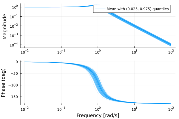
plot(step(G, 0:0.1:20))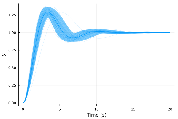
Example: Spinning satellite
This example makes use of real-valued uncertain parameters created using δr, it comes from section 3.7.1 of Skogestad's book.
using RobustAndOptimalControl, ControlSystemsBase, MonteCarloMeasurements, Plots, LinearAlgebra
unsafe_comparisons(true)

a = 10
P = ss([0 a; -a 0], I(2), [1 a; -a 1], 0)
K = ss(1.0I(2))

w = 2π .* exp10.(LinRange(-2, 2, 500))
S, PS, CS, T = gangoffour(P, K)
sigmaplot(S, w, lab="S")
sigmaplot!(T, w, c=2, lab="T", ylims=(0.01, 45))
Both sensitivity functions are very large, expect a non-robust system!
Next, we add parametric uncertainty
a = 10*(1 + 0.1δr(100)) # Create an uncertain parameter with nominal value 10 and 10% uncertainty, represented by 100 samples
P = ss([0 a; -a 0], I(2), [1 a; -a 1], 0)

Sp, PSp, CSp, Tp = gangoffour(P, K)
sigmaplot(Sp, w, lab="S")
sigmaplot!(Tp, w, c=2, lab="T", ylims=(0.01, 100))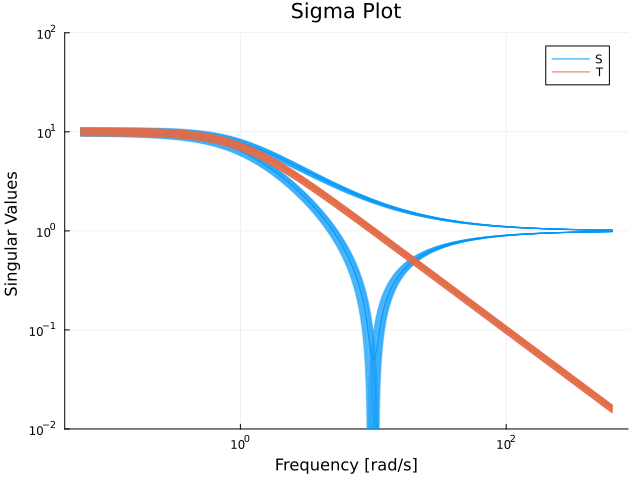
Not only are sensitivity functions large, they vary a lot under the considered uncertainty. We can also plot a step response of one of the sensitivity functions to check how the system behaves
plot(step(c2d(Tp, 0.01), 10))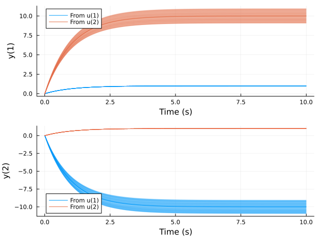
This kind of plot is quite useful, it immediately tells you that this transfer function appears stable, and that there is uncertainty in the static gain etc.
Next, we add complex diagonal multiplicative input uncertainty. With input uncertainty of magnitude $ϵ < \dfrac{1}{σ̄(T)}$ we are guaranteed robust stability (even for “full-block complex perturbations")
a = 10
P = ss([0 a; -a 0], I(2), [1 a; -a 1], 0)

W0 = makeweight(0.2, (20,1), 2)
W = I(2) + W0 .* diagm([δc(100), δc(100)]) # Create a diagonal complex uncertainty weighted in frequency by W0, use 100 samples
Ps = P*W
Ss, PSs, CSs, Ts = gangoffour(Ps, K)
sigmaplot(Ss, w, lab="S")
sigmaplot!(Ts, w, c=2, lab="T", ylims=(0.01, 100))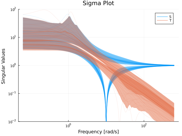
Under this uncertainty, the sensitivity could potentially be sky high., note how some of the 100 realizations peak much higher than the others. This is an indication that the system might be unstable.
With complex entries in the system model, we can't really plot the step response, but we can plot, e.g., the absolute value
res = step(c2d(Ts, 0.01), 10)
plot(res.t, [abs.(res.y)[1,:,1] abs.(res.y)[2,:,2]]) # plot only the diagonal response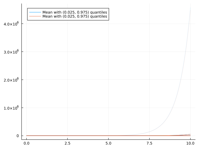
Looks unstable to me. The analysis using $M\Delta$ methodology below will also reach this conclusion.
Example: Distillation Process
This example comes from section 3.7.2 of Skogestad's book. In this example, we'll explore also complex uncertainties, created using δc.
using RobustAndOptimalControl, ControlSystemsBase, MonteCarloMeasurements, Plots, LinearAlgebra
unsafe_comparisons(true)

M = [87.8 -86.4; 108.2 -109.6]
G = Ref(ss(tf(1, [75, 1]))) .* M
RGA = relative_gain_array(G, 0)
sum(abs, RGA) # A good estimate of the true condition number, which is 141.7138.2752186588932large elements in the RGA indicate a process that is difficult to control
We consider the following inverse-based controller, which may also be looked upon as a steady-state decoupler with a PI controller
k1 = 0.7
Kinv = Ref(ss(tf(k1*[75, 1], [1, 0]))) .* inv(M)

# reference filter
F = tf(1, [5, 1]) .* I(2)

w = 2π .* exp10.(LinRange(-2, 2, 500))
sigmaplot(input_sensitivity(G, Kinv), w)
sigmaplot!(output_sensitivity(G, Kinv), w, c=2)
Sensitivity looks nice, how about step response
plot(step(feedback(G*Kinv)*F, 20))
Looks excellent..
We consider again the input gain uncertainty as in the previous example, and we manually select the perturbations to be $ϵ_1 = 0.2$ and $ϵ_2 = 0.2$. We then have
G′ = G * diagm([1 + 0.2, 1 - 0.2])
plot!(step(feedback(G′*Kinv)*F, 20), l=:dash)
Looks very poor! The system was not robust to simultaneous input uncertainty!
We can also do this with a real, diagonal input uncertainty that grows with frequency
W0 = makeweight(0.2, 1, 2.0) # uncertainty goes from 20% at low frequencies to 200% at high frequencies
W = I(2) + W0 .* diagm([δr(100), δr(100)])
Gs = G*W

plot(step(feedback(G*Kinv)*F, 20))
plot!(step(feedback(G′*Kinv)*F, 20), l=:dash)
res = step(c2d(feedback(Gs*Kinv)*F, 0.01), 20)
mcplot!(res.t, abs.(res.y[:, :, 1]'), alpha=0.3)
mcplot!(res.t, abs.(res.y[:, :, 2]'), alpha=0.3)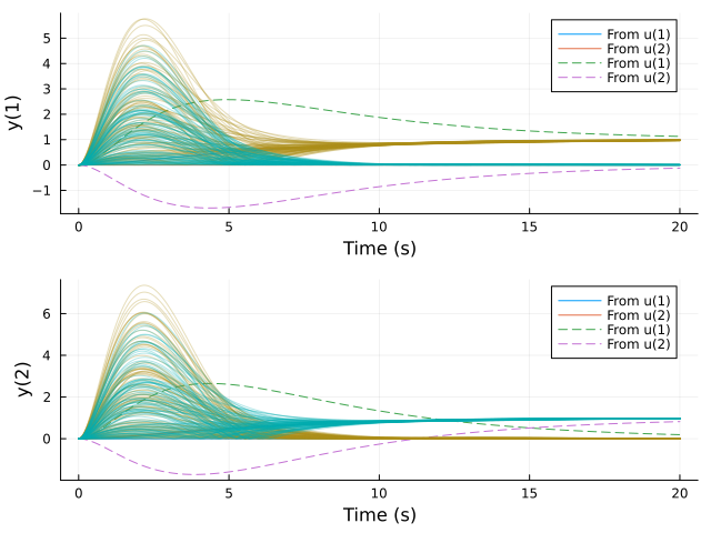
The system is very sensitive to real input uncertainty!
With a complex, diagonal uncertainty, modeling both gain and phase variations, it looks slightly worse, but not much worse than with real uncertainty.
W = I(2) + W0 .* diagm([δc(100), δc(100)]) # note δc instead of δr above
Gs = G*W
res = step(c2d(feedback(Gs*Kinv)*F, 0.01), 20)
mcplot!(res.t, abs.(res.y[:, :, 1]'), alpha=0.3)
mcplot!(res.t, abs.(res.y[:, :, 2]'), alpha=0.3)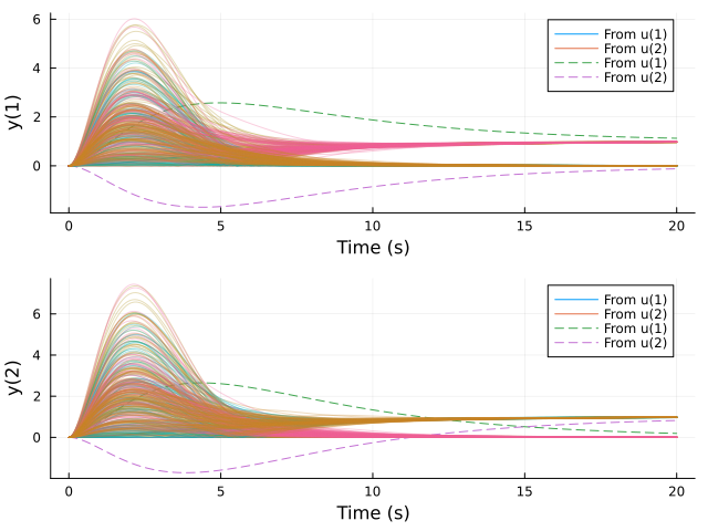
How about the sensitivity functions?
Si = input_sensitivity(Gs, Kinv)
sigmaplot(Si, w, c=1, lab="Si")
So = output_sensitivity(Gs, Kinv)
sigmaplot!(So, w, c=2, lab="So")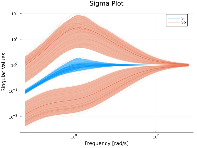
The sensitivity at the plant output is enormous. A low sensitivity with the nominal system does not guarantee robustness!
Model-order reduction for uncertain models
$\nu$-gap approach
The $\nu$-gap metric is a measure of distance between models when they are used in a feedback loop. This metric has the nice property that a controller designed for a process $P$ that achieves a normalized coprime factor margin (ncfmargin) of $m$, will stabilize all models that are within a $\nu$-gap distance of $m$ from $P$. This can be used to reduce the number of uncertain realizations for a model represented with Particles like above in a smart way. Say that we have a plant model $P$
using RobustAndOptimalControl, ControlSystemsBase, MonteCarloMeasurements, Plots
ω = with_nominal(0.9 .. 1.1, 1)
ζ = with_nominal(0.5 ± 0.01, 0.5)
P = tf([ω^2], [1, 2*ζ*ω, ω^2]) |> ss
StateSpace{Continuous, MonteCarloMeasurements.Particles{Float64, 2000}}
A =
-1.0 ± 0.061 -1.0 ± 0.12
1.0 0.0
B =
1.0
0.0
C =
0.0 1.0 ± 0.12
D =
0.0
Continuous-time state-space modelrepresented by 2000 samples (indicated by the displayed type Particles{Float64, 2000}). If we plot $P$, it looks something like this:
w = exp10.(LinRange(-1, 0.5, 150))
# nyquistplot(P, w, lab="Original P", xlims=(-1.1,1.1), ylims=(-1.5,0.7), points=true, format=:png, dpi=80)
bodeplot(P, w, lab="Original P", plotphase = false, format=:png, dpi=80, ri=false, c=1, legend=true)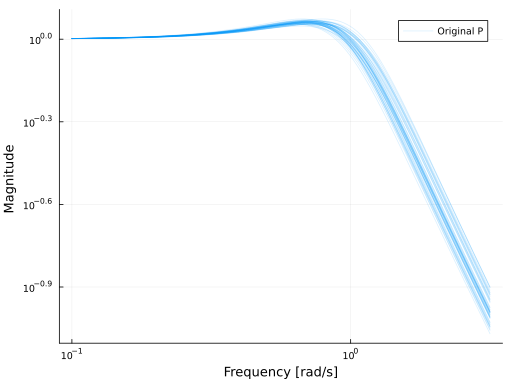
We can compute the $\nu$-gap metric between each realization in $P$ and the nominal value (encoded using with_nominal above):
gap = nugap(P)0.0605788 ± 0.0336 MonteCarloMeasurements.Particles{Float64, 2000}
The worst-case gap is:
pmaximum(gap) # p for "particle" maximum0.12804692157112746That means that if we design a controller for the nominal $P$ without any uncertainty, and make sure that it achieves an ncfmargin of at least this value, it will stabilize all realizations in $P$.
We can also reduce the number of realizations in $P$ by discarding those that are close in the $\nu$-gap sense to the nominal value:
Pr = nu_reduction(P, 0.1)StateSpace{Continuous, MonteCarloMeasurements.Particles{Float64, 319}}
A =
-0.978 ± 0.087 -0.97 ± 0.18
1.0 0.0
B =
1.0
0.0
C =
0.0 0.97 ± 0.18
D =
0.0
Continuous-time state-space modelhere, all realizations that were within a $\nu$-gap distance of 0.1 from the nominal value were discarded. nu_reduction usually reduces the number of realizations substantially. The plot of $P_r$ looks like
# nyquistplot(Pr, lab="Reduced P", xlims=(-1.1,1.1), ylims=(-1.5,0.7), points=true, format=:png, dpi=80)
bodeplot!(Pr, w, lab="Reduced P", plotphase = false, format=:png, dpi=80, ri=false, c=2, l=2)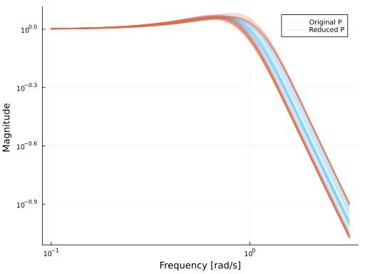
we see that the reduction kept the realizations that were furthest away from the nominal value.
We can reduce the number of realizations even further using nu_reduction_recursive:
Prr = nu_reduction_recursive(P, 0.1)StateSpace{Continuous, MonteCarloMeasurements.Particles{Float64, 3}}
A =
-0.993 ± 0.04 -1.0 ± 0.19
1.0 0.0
B =
1.0
0.0
C =
0.0 1.0 ± 0.19
D =
0.0
Continuous-time state-space model# nyquistplot(Prr, lab="Recursively reduced P", xlims=(-1.1,1.1), ylims=(-1.5,0.7), points=true, format=:png, dpi=80)
bodeplot!(Prr, w, lab="Recursively reduced P", plotphase = false, format=:png, dpi=80, ri=false, c=3, l=3)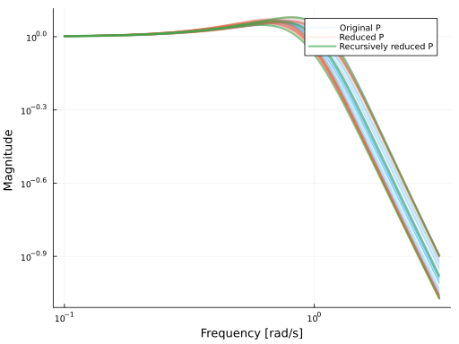
We now have only three realizations left, the nominal one and the two extreme cases (in the $\nu$-gap sense).
The algorithm used in nu_reduction_recursive has a worst-case complexity of $O(N^2)$ where $N$ is the number of realizations (particles) in $P$, but this complexity is only problematic for small gaps and large number of realizations, say, $\nu < 0.02$ and $N > 50$.
With the reduced model, we can more easily perform loop-shaping or other control design tasks, as long as we keep track of ncfmargin staying above our $\nu$-gap.
If P has a stochastic interpretation, i.e., the coefficients come from some distribution, this interpretation will be lost after reduction, mean values and standard deviations will not be preserved. The reduced system should instead be interpreted as preserving worst-case uncertainty.
For more background on the $\nu$-gap metric, see When are two systems similar? and the book by Skogestad and Postlethwaite or by Åström and Murray.
Balanced truncation
Another option to reduce the complexity of an uncertain model is to reinterpret it has a deterministic model with expanded state and output dimensions. For example, an uncertain model with $N$ particles and state and output dimensions $n_x, `n_y$ can be converted into a deterministic model with state and output dimensions $Nn_x$ and $Nn_y$ respectively (the input dimension remains the same). The order of this model can then be reduced using standard balanced truncation (or any other model-reduction method). The conversion from a model with Particles coefficients to an expanded deterministic model is performed by mo_sys_from_particles, and balanced truncation (and other model-reduction techniques) is documented at Model reduction.
Note, the reduced-order model cannot easily be converted back to a representation with Particles when this approach is taken. The model-order reduction will in this case only reduce the state dimension, but the output dimension will remain the same.
We demonstrate this procedure on the model from the section above:
Pmo = mo_sys_from_particles(P, sparse=false)
Pred, S = baltrunc(Pmo)
bodeplot(P, w, lab="Original P", plotphase = false, format=:png, dpi=80, ri=false, c=1, legend=true)
bodeplot!(Pred, w, lab="", plotphase = false, format=:png, dpi=80, c=2, l=1, sp=1, alpha=0.01)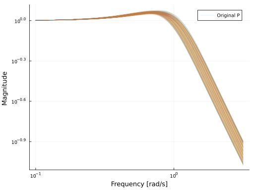
This time, we keep the same output dimension, but the state dimension is reduced significantly:
Pred.nx6Note, Pred here represents the uncertain model with a single deterministic model of order Pred.nx, while the original uncertain model P was represented by 2000 internal models of state dimension 2.
Using the $M\Delta$ framework
The examples above never bothered with things like the "structured singular value", $\mu$ or linear-fractional transforms. We do, however, provide some elementary support for this modeling framework.
In robust control, we often find ourselves having to consider the feedback interconnections below.
        ┌─────────┐
  zΔ◄───┤         │◄────wΔ
        │         │
   z◄───┤    P    │◄────w
        │         │
   y◄───┤         │◄────u
        └─────────┘
┌─────────┐
zΔ◄───┤ │◄────wΔ
│ │
z◄───┤ P │◄────w
│ │
y┌───┤ │◄───┐u
│ └─────────┘ │
│ ┌───┐ │
└─────►│ K ├───────┘
└───┘ ┌───┐
┌─────►│ Δ ├───────┐
│ └───┘ │
│ ┌─────────┐ │
zΔ└───┤ │◄───┘wΔ
│ │
z◄───┤ P │◄────w
│ │
y┌───┤ │◄───┐u
│ └─────────┘ │
│ ┌───┐ │
└─────►│ K ├───────┘
└───┘The first block diagram denotes an open-loop system $P$ with an uncertainty mapping $w_\Delta = \Delta z_\Delta$, a performance mapping from $w$ to $z$ and a input-output mapping between $u$ and $y$. Such a system $P$ can be partitioned as
\[P = \begin{bmatrix} P_{11} & P_{12} & P_{13}\\ P_{21} & P_{22} & P_{23}\\ P_{31} & P_{32} & P_{33}\\ \end{bmatrix}\]
where each $P(s)_{ij}$ is a transfer matrix. The type UncertainSS with constructor uss represents the block
\[P = \begin{bmatrix} P_{11} & P_{12}\\ P_{21} & P_{22}\\ \end{bmatrix}\]
while an ExtendedStateSpace object represents the block
\[P = \begin{bmatrix} P_{22} & P_{23}\\ P_{32} & P_{33}\\ \end{bmatrix}\]
there is thus no type that represents the full system $P$ above. However, we provide the function partition which allows you to convert from a regular statespace system to an extended statespace object, and it is thus possible to represent $P$ by placing the whole block
\[P = \begin{bmatrix} P_{22} & P_{23}\\ P_{32} & P_{33}\\ \end{bmatrix}\]
into $P_{22}$ for the purposes of uncertainty analysis (use ss to convert it to a standard statespace object), and later use partition to recover the internal block structure.
Given an UncertainSS $P$, we can close the loop around $\Delta$ by calling lft(P, Δ, :u), and given an ExtendedStateSpace, we can close the loop around K by calling starprod(P, K) or lft(P, K) (using positive feedback). This works even if P is a regular statespace object, in which case the convention is that the inputs and outputs are ordered as in the block diagrams above. The number of signals that will be connected by lft is determined by the input-output arity of $K$ and $\Delta$ respectively.
We have the following methods for lft (in addition to the standard ones in ControlSystemsBase.jl)
lft(G::UncertainSS, K::LTISystem)forms the lower LFT closing the loop around $K$.lft(G::UncertainSS, Δ::AbstractArray=G.Δ)forms the upper LFT closing the loop around $\Delta$.lft(G::ExtendedStateSpace, K)forms the lower LFT closing the loop around $K$.
Robust stability and performance
To check robust stability of the system in the last block diagram (with or without $z$ and $w$), we can use the functions structured_singular_value, robstab and diskmargin.
Currently, structured_singular_value is rather limited and supports diagonal complex blocks only. If $\Delta$ is a single full complex block, opnorm(P.M) < 1 is the condition for stability.
Robust performance can be verified by introducing an additional fictitious "performance perturbation" $\Delta_p$ which is a full complex block, around which we close the loop from $z$ to $w$ and check the structured_singular_value with the augmented perturbation block
\[\Delta_a = \begin{bmatrix} \Delta & 0\\ 0 & \Delta_p\\ \end{bmatrix}\]
Examples
We repeat the first example here, but using $M\Delta$ formalism rather than direct Monte-Carlo modeling.
When we call δc without any arguments, we get a symbolic (or structured) representation of the uncertainty rather than the sampled representation we got from calling δc(100).
a = 10
P = ss([0 a; -a 0], I(2), [1 a; -a 1], 0)
W0 = makeweight(0.2, (1,1), 2) |> ss
W = I(2) + W0 .* uss([δc(), δc()]) # Create a diagonal complex uncertainty weighted in frequency by W0
Ps = P*W
UncertainSS{Continuous}
A =
0.0 10.0 -1.590990257669732 0.0
-10.0 0.0 0.0 -1.590990257669732
0.0 0.0 -1.7677669529663689 0.0
0.0 0.0 0.0 -1.7677669529663689
B =
2.0 0.0 1.0 0.0
0.0 2.0 0.0 1.0
2.0 0.0 0.0 0.0
0.0 2.0 0.0 0.0
C =
0.0 0.0 0.0 0.0
0.0 0.0 0.0 0.0
1.0 10.0 0.0 0.0
-10.0 1.0 0.0 0.0
D =
0.0 0.0 1.0 0.0
0.0 0.0 0.0 1.0
0.0 0.0 0.0 0.0
0.0 0.0 0.0 0.0
Continuous-time state-space modelPs is now represented as a upper linear fractional transform (upper LFT).
We can draw samples from this uncertainty representation (sampling of $\Delta$ and closing the loop starprod(Δ, Ps)) like so
Psamples = rand(Ps, 100)
sigmaplot(Psamples, w)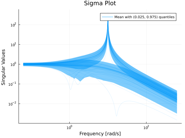
We can extract the nominal model using
system_mapping(Ps)StateSpace{Continuous, Float64}
A =
0.0 10.0
-10.0 0.0
B =
1.0 0.0
0.0 1.0
C =
1.0 10.0
-10.0 1.0
D =
0.0 0.0
0.0 0.0
Continuous-time state-space modelAnd obtain $M$ and $\Delta$ when the loop is closed with $K$ like this:
lft(Ps, K).MStateSpace{Continuous, Float64}
A =
1.0 20.0 -1.590990257669732 0.0
-20.0 1.0 0.0 -1.590990257669732
0.0 0.0 -1.7677669529663689 0.0
0.0 0.0 0.0 -1.7677669529663689
B =
2.0 0.0
0.0 2.0
2.0 0.0
0.0 2.0
C =
1.0 10.0 0.0 0.0
-10.0 1.0 0.0 0.0
D =
0.0 0.0
0.0 0.0
Continuous-time state-space modelPs.Δ # Ps.delta also works2-element Vector{Any}:
δ{ComplexF64, Float64}(0.0 + 0.0im, 1.0, Symbol("##δ#507"))
δ{ComplexF64, Float64}(0.0 + 0.0im, 1.0, Symbol("##δ#508"))We can evaluate the frequency response of $M$ and calculate the structured singular value $\mu$
M = freqresp(lft(Ps, -K).M, w) # -K to get negative feedback
μ = structured_singular_value(M)
plot(w, μ, xscale=:log10, title="Structured singular value μ", xlabel="Frequency [rad/s]", ylabel="μ")
$\mu$ is very high, whenever $\mu > 1$, the system is not stable with respect to the modeled uncertainty. The tolerated uncertainty is only about $\dfrac{1}{||\mu||_\infty}$
1/norm(μ, Inf)0.13647901995727751of the modeled uncertainty. Another way of calculating this value is
robstab(lft(Ps, -K))0.136477575525228Internals of the $M\Delta$ framework
TODO
Uncertain time delays
Modeling uncertain time delays can be done in several ways, one approach is to make use of a multiplicative uncertainty weight created using neglected_delay multiplied by an uncertain element created using δc, example:
using RobustAndOptimalControl, ControlSystemsBase, MonteCarloMeasurements, Plots, LinearAlgebra
a  = 10
P  = ss([0 a; -a 0], I(2), [1 a; -a 1], 0) # Plant
W0 = neglected_delay(0.005) |> ss # Weight
W  = I(2) + W0 .* uss([δc(), δc()]) # Create a diagonal real uncertainty weighted in frequency by W0
Ps = P*W # Uncertain plant
Psamples = rand(Ps, 1000) # Sample the uncertain plant for plotting
w = exp10.(LinRange(-1, 3, 300)) # Frequency vector
bodeplot(Psamples, w, legend=false, N=0, quantile=0)
bodeplot!(P*[delay(0.005) tf(0); tf(0) delay(0.005)], w) # Compare to the plant with a model of the delay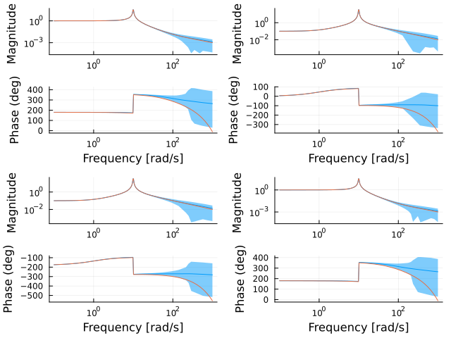
We see that the uncertain model set includes the model with the delay. Note how this approximation approach imparts some uncertainty also in the gain.
More details on this approach can be found in Skogestad sec. 7.4.
The other alternative is to use use sampled uncertain delays. The next example shows how we can create a system with an uncertain delay, where we know that the delay is an integer number of milliseconds between 1ms and 4ms.
using RobustAndOptimalControl, ControlSystemsBase, MonteCarloMeasurements, Plots, LinearAlgebra
unsafe_comparisons(true)
L = Particles(collect((1:4) ./ 1000)) # Uncertain time delay, an integer number of milliseconds between 1ms and 4ms
P = delay(L)*tf(1, [0.01, 1])
C = pid(2, 1)
w = exp10.(-1:0.01:4)
plot(
     bodeplot(P, exp10.(-1:0.001:3), legend=false),
     # plot(step(feedback(P, C), 0:0.0001:0.05), lab="L = " .* string.(P.Tau[].particles'), title="Disturbance response"), # This simulation requires using ControlSystems
     nyquistplot(P*C, w[1:10:end], points=true, xlims=(-3.5, 2.5), ylims=(-5, 1.5), Ms_circles=[1.5, 2], alpha=1) # Note, the nyquistplot with uncertain coefficients requires manual selection of plot limits
)
Notice how the gain is completely certain, while the phase starts becoming very uncertain for high frequencies.
Models of uncertain dynamics
This section goes through a number of uncertainty descriptions in block-diagram form and shows the equivalent transfer function appearing in feedback with the uncertain element. A common approach is to model an uncertain element as $W(s)\Delta$ where $||\Delta|| \leq 1$ and $W(s)$ is a frequency-dependent weighting function that is large for frequencies where the uncertainty is large.
Additive uncertainty
          ┌────┐         ┌────┐
        ┌►│ WΔ ├─┐    ┌─►│ WΔ ├──┐
        │ └────┘ │    │  └────┘  │
        │        │    │          │
  ┌───┐ │  ┌───┐ ▼    │ ┌──────┐ │
┌►│ C ├─┴─►│ P ├─+    │ │  C   │ │
│ └───┘    └───┘ │    └─┤ ──── │◄┘
│                │      │ I+PC │
└────────────────┘      └──────┘
The system is made robust with respect to this uncertainty by making
\[W\dfrac{C}{I+PC} < 1\]
for all frequencies.
Multiplicative uncertainty
At the process output
                  ┌────┐          ┌────┐
                ┌►│ WΔ ├┐      ┌─►│ WΔ ├──┐
                │ └────┘│      │  └────┘  │
  ┌───┐   ┌───┐ │       ▼      │          │
┌►│ C ├──►│ P ├─┴───────+─►    │ ┌──────┐ │
│ └───┘   └───┘         │      │ │  PC  │ │
│                       │      └─┤ ──── │◄┘
└───────────────────────┘        │ I+PC │
                                 └──────┘
The system is made robust with respect to this uncertainty by making the complimentary sensitivity function $T$ satisfy
\[W\dfrac{PC}{I+PC} = WT < 1\]
for all frequencies.
This means that we must make the transfer function $T$ small for frequencies where the relative uncertainty is large. The relative uncertainty is always > 1 for sufficiently large frequencies, and this gives rise to the common adage of "apply lowpass filtering to avoid exciting higher-order dynamics at high frequencies".
This uncertainty representation was used in the examples above where we spoke about multiplicative uncertainty. For MIMO systems, uncertainty appearing on the plant input may behave different than if it appears on the plant output. In general, the loop-transfer function $L_o = PC$ denotes the output loop-transfer function (the loop is broken at the output of the plant) and $L_i = CP$ denotes the input loop-transfer function (the loop is broken at the input of the plant). For multiplicative uncertainty at the plant input, the corresponding transfer function to be constrained is
\[\dfrac{CP}{I+CP}W_i = TW_i < 1\]
with corresponding diagram
          ┌───┐                  ┌────┐
        ┌►│ ΔW├─┐             ┌─►│ ΔW ├───┐
        │ └───┘ │             │  └────┘   │
        │       │             │           │
  ┌───┐ │       ▼  ┌───┐      │ ┌──────┐  │
┌►│ C ├─┴─────────►│ P ├─┐    │ │  CP  │  │
│ └───┘            └───┘ │    └─┤ ──── │◄─┘
│                        │      │ I+CP │
└────────────────────────┘      └──────┘
The input version represents uncertainty in the actuator, and is a particularly attractive object for analysis of SIMO systems, where this transfer function is SISO.
Skogestad and Postlethwaite Sec. 7.5.1
Example
See the example with Uncertain time delays above.
Additive feedback uncertainty
          ┌────┐        ┌────┐
        ┌─┤ WΔ │◄┐   ┌─►│ WΔ ├──┐
        │ └────┘ │   │  └────┘  │
        │        │   │          │
  ┌───┐ ▼  ┌───┐ │   │ ┌──────┐ │
┌►│ C ├─+─►│ P ├─┤   │ │  P   │ │
│ └───┘    └───┘ │   └─┤ ──── │◄┘
│                │     │ I+PC │
└────────────────┘     └──────┘
The system is made robust with respect to this uncertainty by making
\[W\dfrac{P}{I+PC} < 1\]
for all frequencies.
This kind of uncertainty can represent uncertainty regarding presence of feedback loops, and uncertainty regarding the implementation of the controller (this uncertainty is equivalent to additive uncertainty in the controller).
Multiplicative feedback uncertainty
At the process output
                 ┌────┐           ┌────┐
                ┌┤ WΔ │◄┐      ┌─►│ WΔ ├──┐
                │└────┘ │      │  └────┘  │
  ┌───┐   ┌───┐ ▼       │      │          │
┌►│ C ├──►│ P ├─+───────┼─►    │ ┌──────┐ │
│ └───┘   └───┘         │      │ │  I   │ │
│                       │      └─┤ ──── │◄┘
└───────────────────────┘        │ I+PC │
                                 └──────┘
The system is made robust with respect to this uncertainty by making the (output) sensitivity function $S$ satisfy
\[W\dfrac{I}{I+PC} = WS < 1\]
for all frequencies.
This kind of uncertainty can represent uncertainty regarding which half plane poles are located. For frequencies where $W$ is larger than 1, poles can move from the left to the right half plane, and we thus need to make $S$ small (use lots of feedback) for those frequencies.
At the process input:
          ┌────┐                  ┌───┐
        ┌─┤ WΔ │◄┐             ┌─►│ WΔ├───┐
        │ └────┘ │             │  └───┘   │
        │        │             │          │
  ┌───┐ ▼        │  ┌───┐      │ ┌──────┐ │
┌►│ C ├─+────────┴─►│ P ├┐     │ │  I   │ │
│ └───┘             └───┘│     └─┤ ──── │◄┘
│                        │       │ I+CP │
└────────────────────────┘       └──────┘
The system is made robust with respect to this uncertainty by making the (input) sensitivity function $S_i$ satisfy
\[\dfrac{I}{I+CP} W = S_i W < 1\]
for all frequencies.
Skogestad and Postlethwaite Sec. 7.5.3
Uncertainty through disturbances
Uncertainty can of course also be modeled as disturbances acting on the system. Similar to above, we may model disturbances as a signal that has $L_2$ norm less than 1, scaled by a weight $W(s)$. Additive, norm-bounded disturbances can never make a stable linear system unstable, the uncertainty does not appear *in the loop. The analysis of such disturbances can thus be focused on making the transfer function from the disturbance to the performance output small.
Some convenient facts when working with disturbances are that the $H_\infty$ norm of a transfer function $e = G_{ed}d$ is equal to the worst-case gain in $L_2$ norm of signals
\[\|G_{ed}\|_\infty = \sup_{d} \dfrac{||e||_2}{||d||_2}\]
and that the $H_2$ norm is equal to the gain in variance
\[\sigma_e^2 = \|G_{ed}\|_2 \sigma_d^2\]
Visualizing uncertainty
For any of the uncertainty descriptions above, we may plot the total loop gain excluding the uncertain element $\Delta$, that is, the weight $W(s)$ multiplied by the equivalent transfer function of the nominal part of the loop. For example, for multiplicative uncertainty at the plant output, we would plot $WT$ in a sigmaplot and verify that all singular values are smaller than 1 for all frequencies. Alternatively, for SISO systems, we may plot $T$ and $W^{-1}$ in a Bode plot and verify that $T < W^{-1}$ for all frequencies. This latter visualization usually provides better intuition.
Example: Bode plot
Below, we perform this procedure for an multiplicative (relative) uncertainty model at the plant output. The uncertainty weight $W(s)$ is chosen to give 10% uncertainty at low frequencies and 10x uncertainty at high frequencies, indicating that we are absolutely oblivious to the behavior of the plant at high frequencies. This is often the case, either because identification experiments did not contain excitation for high frequencies, or because the plant had nonlinear behavior at higher frequencies.
using ControlSystemsBase, RobustAndOptimalControl, Plots
P = tf(1, [1, 2, 1]) # Plant model
C = pid(19.5, 0)      # Controller
W = makeweight(0.1, 10, 10) # Low uncertainty (0.1) at low frequencies, large (10) at high frequencies.
bodeplot([comp_sensitivity(P, C), inv(W)], lab=["\$S\$" "\$W^{-1}\$"], linestyle=[:solid :dash], plotphase=false)
As long as the complimentary sensitivity function $T(s)$ stays below the inverse weight $W^{-1}(s)$, the closed-loop system is robust with respect to the modeled uncertainty.
Example: Nyquist plot
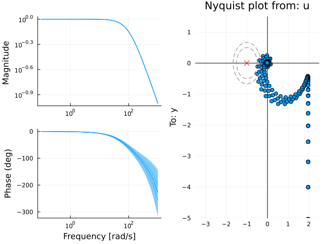
Continuing from the Bode-plot example above, we can translate the multiplicative weight $W(s)$ to a set of circles we could plot in the Nyquist diagram, one for each frequency, that covers the true open-loop system. For sampled representations of uncertainty, this is done using fit_complex_perturbations, but here, we do it manually. For a given frequency $\omega$, the radius of the circle for an additive uncertainty in the loop gain is given by $|W(i\omega)|$, and for a multiplicative (relative) uncertainty, it is scaled by the loop gain $|W(i\omega) P(i\omega) C(i\omega)|$.[circ] The center of the circle is simply given by the nominal value of the loop-gain $P(i\omega)C(i\omega)$.
w = exp10.(LinRange(-2, 2, 200))
centers = freqrespv(P*C, w)
radii = abs.(freqrespv(W*P*C, w))
nyquistplot(P*C, w, xlims=(-4,0.1), ylims=(-4,0.1))
nyquistcircles!(w, centers, radii)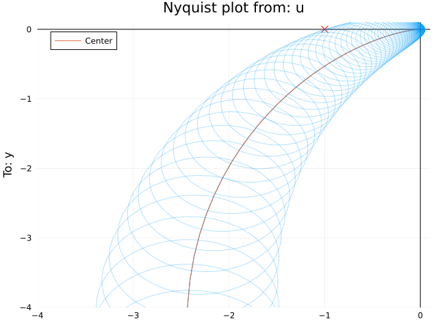
If the plots above are created using the plotly() backend, each circle is associated with hover information that is accessible by hovering the mouse over the plot. This indicates that the circle that touches the critical point is the one at $\omega \approx 4.5$, which coincides exactly with the point at thich the Bode plot above touches the inverse weight$W^{-1}$.
Converting between uncertainty descriptions
Any of the representations above, if modeled using uncertainty elements (UncertainSS, δc, δr), may be converted to a sampled uncertainty representation using rand(P_uncertain, 100). The sampled representation can be further converted using fit_complex_perturbations which results in a set of circles, additive or multiplicative (relative), one for each frequency considered, that covers the true system. These can be plotted in a Nyquist diagram using nyquistcircles (see Example: Nyquist plot above).
A sampled representation can also be converted to a nominal value and a maximum $\nu$-gap, see Model-order reduction for uncertain models for an example of this
More references
Skogestad Sec. 8.5.3 contains result for moving uncertainty descriptions between input and output for MIMO systems as well as some additional forms of uncertainty descriptions, with robust stability conditions listed in Sec. 8.6.1.
- SkogestadSkogestad, "Multivariable Feedback Control: Analysis and Design"
- Doyle91Doyle, Packard, Zhou, "Review of LFTs, LMIs and μ".
https://www.researchgate.net/publication/257200344_Review_of_LFTs_LMIs_and_mu - circA relative uncertainty does not apply to $P$ only, it appears after $P$ and thus models the relative uncertainty in the entire loop gain $PC$.