ControlSystemsBase.bodeplotControlSystemsBase.gangoffourplotControlSystemsBase.marginplotControlSystemsBase.nicholsplotControlSystemsBase.nyquistplotControlSystemsBase.pzmapControlSystemsBase.rgaplotControlSystemsBase.rlocusplotControlSystemsBase.setPlotScaleControlSystemsBase.sigmaplot
All plotting requires the user to manually load the Plots.jl library, e.g., by calling using Plots. See also experimental Makie support below.
Plotting functions
ControlSystemsBase.bodeplot — Function
fig = bodeplot(sys, args...)
bodeplot(LTISystem[sys1, sys2...], args...; plotphase=true, balance = true, kwargs...)
Create a Bode plot of the LTISystem(s). A frequency vector w can be optionally provided. To change the Magnitude scale see setPlotScale. The default magnitude scale is "log10" (absolute scale).
- If
hz=true, the plot x-axis will be displayed in Hertz, the input frequency vector is still treated as rad/s. balance: Callbalance_statespaceon the system before plotting.adjust_phase_start: If true, the phase will be adjusted so that it starts at -90*intexcess degrees, whereintexcessis the integrator excess of the system.adaptive: If true, an adaptive frequency grid is used in order to keep the number of plotted points low, while resolving features in the frequency response well. If a manually provided frequency vector is used, this may be downsampled before plotting.
kwargs is sent as argument to RecipesBase.plot.
ControlSystemsBase.gangoffourplot — Method
fig = gangoffourplot(P::LTISystem, C::LTISystem; minimal=true, plotphase=false, Ms_lines = [1.0, 1.25, 1.5], Mt_lines = [], sigma = true, kwargs...)Gang-of-Four plot.
sigma determines whether a sigmaplot is used instead of a bodeplot for MIMO S and T. kwargs are sent as argument to RecipesBase.plot.
ControlSystemsBase.marginplot — Function
fig = marginplot(sys::LTISystem [,w::AbstractVector]; hz=false, balance=true, kwargs...)
marginplot(sys::Vector{LTISystem}, w::AbstractVector; hz=false, balance=true, kwargs...)
Plot all the amplitude and phase margins of the system(s) sys.
- A frequency vector
wcan be optionally provided. hz: If true, the plot x-axis will be displayed in Hertz, the input frequency vector is still treated as rad/s.balance: Callbalance_statespaceon the system before plotting.adjust_phase_start: If true, the phase will be adjusted so that it starts at -90*intexcess degrees, whereintexcessis the integrator excess of the system.
kwargs is sent as argument to RecipesBase.plot.
ControlSystemsBase.nicholsplot — Function
fig = nicholsplot{T<:LTISystem}(systems::Vector{T}, w::AbstractVector; kwargs...)Create a Nichols plot of the LTISystem(s). A frequency vector w can be optionally provided.
Keyword arguments:
text = true
Gains = [12, 6, 3, 1, 0.5, -0.5, -1, -3, -6, -10, -20, -40, -60]
pInc = 30
sat = 0.4
val = 0.85
fontsize = 10
pInc determines the increment in degrees between phase lines.
sat ∈ [0,1] determines the saturation of the gain lines
val ∈ [0,1] determines the brightness of the gain lines
Additional keyword arguments are sent to the function plotting the systems and can be used to specify colors, line styles etc. using regular RecipesBase.jl syntax
This function is based on code subject to the two-clause BSD licence Copyright 2011 Will Robertson Copyright 2011 Philipp Allgeuer
ControlSystemsBase.nyquistplot — Function
fig = nyquistplot(sys;                Ms_circles=Float64[], Mt_circles=Float64[], disk_margin_circles=Float64[], unit_circle=false, hz=false, critical_point=-1, kwargs...)
nyquistplot(LTISystem[sys1, sys2...]; Ms_circles=Float64[], Mt_circles=Float64[], disk_margin_circles=Float64[], unit_circle=false, hz=false, critical_point=-1, kwargs...)
Create a Nyquist plot of the LTISystem(s). A frequency vector w can be optionally provided.
unit_circle: if the unit circle should be displayed. The Nyquist curve crosses the unit circle at the gain crossover frequency.Ms_circles: draw circles corresponding to given levels of sensitivity (circles around -1 with radii1/Ms).Ms_circlescan be supplied as a number or a vector of numbers. A design staying outside such a circle has a phase margin of at least2asin(1/(2Ms))rad and a gain margin of at leastMs/(Ms-1). See alsomargin_bounds,Ms_from_phase_marginandMs_from_gain_margin.Mt_circles: draw circles corresponding to given levels of complementary sensitivity.Mt_circlescan be supplied as a number or a vector of numbers.disk_margin_circles: draw disk-margin circles for the given values ofM(M > 1, supplied as a number or vector of numbers). Each circle is the disk on the negative real axis passing through-(M-1)/Mand-M/(M-1). A design whose Nyquist curve stays outside this disk has a symmetric (balanced) gain margin of at least[(M-1)/M, M/(M-1)]— i.e. the loop gain may be multiplied by any real factor in that interval without losing stability — together with a phase margin of at leastatan((2M-1)/(2M(M-1)))rad. LargerMcorresponds to a smaller, more permissive disk and weaker margin guarantees.critical_point: point on real axis to mark as critical for encirclements- If
hz=true, the hover information will be displayed in Hertz, the input frequency vector is still treated as rad/s. balance: Callbalance_statespaceon the system before plotting.
kwargs is sent as argument to plot.
ControlSystemsBase.pzmap — Function
fig = pzmap(fig, system, args...; hz = false, kwargs...)Create a pole-zero map of the LTISystem(s) in figure fig, args and kwargs will be sent to the scatter plot command.
To customize the unit-circle drawn for discrete systems, modify the line attributes, e.g., linecolor=:red.
If hz is true, all poles and zeros are scaled by 1/2π.
ControlSystemsBase.rgaplot — Function
rgaplot(sys, args...; hz=false)
rgaplot(LTISystem[sys1, sys2...], args...; hz=false, balance=true)
Plot the relative-gain array entries of the LTISystem(s). A frequency vector w can be optionally provided.
- If
hz=true, the plot x-axis will be displayed in Hertz, the input frequency vector is still treated as rad/s. balance: Callbalance_statespaceon the system before plotting.
kwargs is sent as argument to Plots.plot.
ControlSystemsBase.setPlotScale — Method
setPlotScale(str)Set the default scale of magnitude in bodeplot and sigmaplot. str should be either "dB" or "log10". The default scale if none is chosen is "log10".
ControlSystemsBase.sigmaplot — Function
sigmaplot(sys, args...; hz=false balance=true, extrema)
sigmaplot(LTISystem[sys1, sys2...], args...; hz=false, balance=true, extrema)
Plot the singular values of the frequency response of the LTISystem(s). A frequency vector w can be optionally provided.
- If
hz=true, the plot x-axis will be displayed in Hertz, the input frequency vector is still treated as rad/s. balance: Callbalance_statespaceon the system before plotting.extrema: Only plot the largest and smallest singular values.
kwargs is sent as argument to Plots.plot.
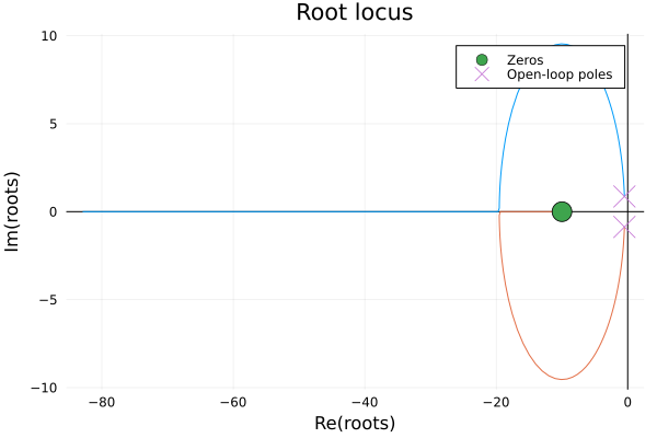
ControlSystemsBase.rlocusplot — Function
rlocusplot(siso_sys)
rlocusplot(sys::StateSpace, K::Matrix; output=false)
Plot the root locus of a system under feedback.
If a SISO system is passed, the feedback gain K is a scalar that ranges from 0 to K (if provided). If a StateSpace system is passed, K is a matrix that defines the feedback gain, and the poles are computed as K ranges from 0*K to 1*K. In this case, K is assumed to be a state-feedback matrix of dimension (nu, nx). To compute the poles for output feedback, pass output = true and K of dimension (nu, ny).
- To plot simulation results such as step and impulse responses, use
plot(::SimResult), see alsolsim.
Examples
Bode plot

tf1 = tf([1],[1,1])
tf2 = tf([1/5,2],[1,1,1])
sys = [tf1 tf2]
ws = exp10.(range(-2,stop=2,length=200))
bodeplot(sys, ws)
Sigma plot
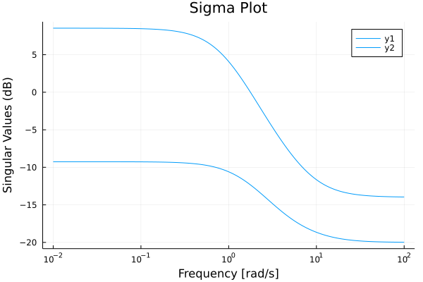
sys = ss([-1 2; 0 1], [1 0; 1 1], [1 0; 0 1], [0.1 0; 0 -0.2])
sigmaplot(sys)
Margin

tf1 = tf([1],[1,1])
tf2 = tf([1/5,2],[1,1,1])
ws = exp10.(range(-2,stop=2,length=200))
marginplot([tf1, tf2], ws)
Gangoffour plot
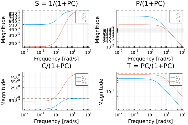
tf1 = tf([1.0],[1,1])
gangoffourplot(tf1, [tf(1), tf(5)])
Nyquist plot

sys = ss([-1 2; 0 1], [1 0; 1 1], [1 0; 0 1], [0.1 0; 0 -0.2])
ws = exp10.(range(-2,stop=2,length=200))
nyquistplot(sys, ws, Ms_circles=1.2, Mt_circles=1.2)
Nichols plot
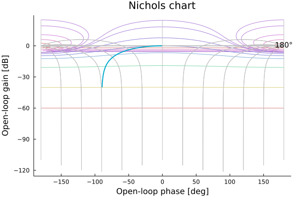
tf1 = tf([1],[1,1])
ws = exp10.(range(-2,stop=2,length=200))
nicholsplot(tf1,ws)
Pole-zero plot
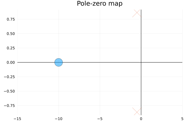
tf2 = tf([1/5,2],[1,1,1])
pzmap(c2d(tf2, 0.1))
Rlocus plot
Lsim response plot
Simulation results are plotted directly using the plot function: 
sys = ss([-1 2; 0 1], [1 0; 1 1], [1 0; 0 1], [0.1 0; 0 -0.2])
sysd = c2d(sys, 0.01)
L = lqr(sysd, [1 0; 0 1], [1 0; 0 1])
ts = 0:0.01:5
plot(lsim(sysd, (x,i)->-L*x, ts; x0=[1;2]), plotu=true)
Impulse response plot
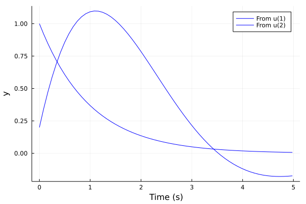
tf1 = tf([1],[1,1])
tf2 = tf([1/5,2],[1,1,1])
sys = [tf1 tf2]
sysd = c2d(ss(sys), 0.01)
plot(impulse(sysd, 5), l=:blue)
Step response plot
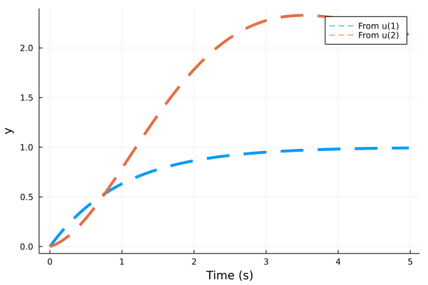
tf1 = tf([1],[1,1])
tf2 = tf([1/5,2],[1,1,1])
sys = [tf1 tf2]
sysd = c2d(ss(sys), 0.01)
res = step(sysd, 5)
plot(res, l=(:dash, 4))
# plot!(stepinfo(step(sysd[1,1], 10))) # adds extra info to the plot
Makie support
The support for plotting with Makie is currently experimental and at any time subject to breaking changes or removal not respecting semantic versioning.
ControlSystemsBase provides experimental support for plotting with Makie.jl through the CSMakie module. This support is loaded automatically when you load a Makie backend (GLMakie, CairoMakie, or WGLMakie).
Usage
using ControlSystemsBase, GLMakie  # or CairoMakie, WGLMakie

# Create a system
P = tf([1], [1, 2, 1])

# Use CSMakie plotting functions
CSMakie.bodeplot(P)
CSMakie.nyquistplot(P)
CSMakie.pzmap(P)
# ... and more

# Direct plotting of simulation results
res = step(P, 10)
plot(res)  # Creates a figure with time-domain response (note that this function does not belong to the CSMakie module)

si = stepinfo(res)
plot(si)  # Visualizes step response characteristics
Available functions
The CSMakie module provides Makie implementations of the following plotting functions:
CSMakie.bodeplot- Bode magnitude and phase plotsCSMakie.nyquistplot- Nyquist plots with optional M and Mt circlesCSMakie.sigmaplot- Singular value plotsCSMakie.marginplot- Gain and phase margin plotsCSMakie.pzmap- Pole-zero mapsCSMakie.nicholsplot- Nichols chartsCSMakie.rgaplot- Relative gain array plotsCSMakie.rlocusplot- Root locus plotsCSMakie.leadlinkcurve- Lead-link design curves
Additionally, SimResult and StepInfo types can be plotted directly using Makie's plot function.