Performance considerations

Numerical accuracy

Transfer functions, and indeed polynomials in general, are infamous for having poor numerical properties and for this reason, it's ill-advised to use high-order transfer functions. Orders as low as 6 may already be considered high. When a transfer function is converted to a state-space representation using ss(G), balancing is automatically performed in an attempt at making the numerical properties of the model better.

This problem is illustrated below, where we first create a statespace system $G$ and convert this to a transfer function $G_1$. We then perturb a single element of the dynamics matrix $A$ by adding the machine epsilon for Float64 (eps() = 2.22044e-16), and convert this perturbed statespace system to a transfer function $G_2$. The difference between the two transfer functions is enormous, the norm of the difference in their denominator coefficient vectors is on the order of $10^{96}$.

sys = ssrand(1,1,100);
G1 = tf(sys);
sys.A[1,1] += eps();
G2 = tf(sys);
norm(denvec(G1)[] - denvec(G2)[])
6.270683106765845e96

If we plot the poles of the two systems, they are also very different

scatter(poles(G1)); scatter!(poles(G2))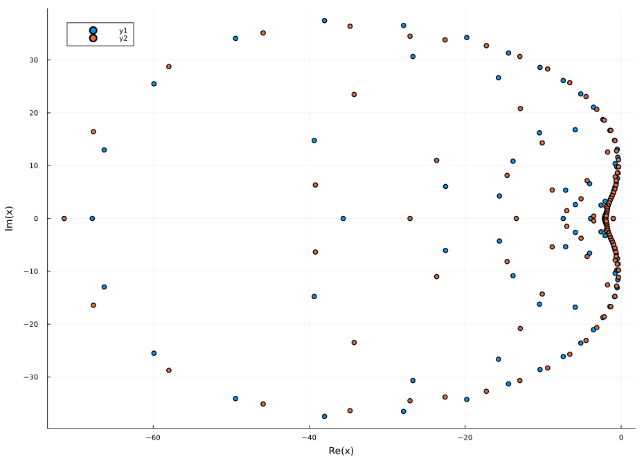

If we instead compute the poles of the statespace model before and after the perturbation, they are almost indistinguishable.

State-space balancing

The function balance_statespace can be used to compute a balancing transformation $T$ that attempts to scale the system so that the row and column norms of

\[\begin{bmatrix} TAT^{-1} & TB\\ CT^{-1} & 0 \end{bmatrix}\]

are approximately equal. This typically improves the numerical performance of several algorithms, including frequency-response calculations and continuous-time simulations. When frequency-responses are plotted using any of the built-in functions, such as bodeplot or nyquistplot, this balancing is performed automatically. However, when calling bode and nyquist directly, the user is responsible for performing the balancing. The balancing is a relatively cheap operation, but it

1. Changes the state representations of the system (but not the input-output mapping). If balancing is performed before simulation, the output will correspond to the output of the original system, but the state trajectory will not.
2. Allocates some memory.

Balancing is also automatically performed when a transfer function is converted to a statespace system using ss(G), to convert without balancing, call convert(StateSpace, G, balance=false).

Intuitively (and simplified), balancing may be beneficial when the magnitude of the elements of the $B$ matrix are vastly different from the magnitudes of the element of the $C$ matrix, or when the $A$ matrix contains very large coefficients. An example that exhibits all of these traits is the following

using ControlSystemsBase, LinearAlgebra
A = [-6.537773175952662 0.0 0.0 0.0 -9.892378564622923e-9 0.0; 0.0 -6.537773175952662 0.0 0.0 0.0 -9.892378564622923e-9; 2.0163803998106024e8 2.0163803998106024e8 -0.006223894167415392 -1.551620418759878e8 0.002358202548321148 0.002358202548321148; 0.0 0.0 5.063545034365582e-9 -0.4479539754649166 0.0 0.0; -2.824060629317756e8 2.0198389074625736e8 -0.006234569427701143 -1.5542817673286995e8 -0.7305736722226711 0.0023622473513548576; 2.0198389074625736e8 -2.824060629317756e8 -0.006234569427701143 -1.5542817673286995e8 0.0023622473513548576 -0.7305736722226711]
B = [0.004019511633336128; 0.004019511633336128; 0.0; 0.0; 297809.51426114445; 297809.51426114445]
C = [0.0 0.0 0.0 1.0 0.0 0.0]
D = [0.0]
linsys = ss(A,B,C,D)
norm(linsys.A, Inf), norm(linsys.B, Inf), norm(linsys.C, Inf)

(2.824060629317756e8, 297809.51426114445, 1.0)

which after balancing becomes

bsys, T = balance_statespace(linsys)
norm(bsys.A, Inf), norm(bsys.B, Inf), norm(bsys.C, Inf)

(6.537773175952662, 0.032156093066689026, 0.0625)

If you plot the frequency-response of the two systems using bodeplot, you'll see that they differ significantly (the balanced one is correct).

Frequency-response calculation

For small systems (small number of inputs, outputs and states), evaluating the frequency-response of a transfer function is reasonably accurate and very fast.

G = tf(1, [1, 1])
w = exp10.(LinRange(-2, 2, 200));
@btime freqresp($G, $w);
# 4.351 μs (2 allocations: 3.31 KiB)

Evaluating the frequency-response for the equivalent state-space system incurs some additional allocations due to a Hessenberg matrix factorization

sys = ss(G);
@btime freqresp($sys, $w);
# 20.820 μs (16 allocations: 37.20 KiB)

For larger systems, the state-space calculations are considerably more accurate, provided that the realization is well balanced.

For optimal performance, one may preallocate the return array

ny,nu = size(G)
R = zeros(ComplexF64, ny, nu, length(w));

@btime freqresp!($R, $G, $w);
# 4.214 μs (1 allocation: 64 bytes)

Other functions that accept preallocated workspaces are

• bodemag!
• freqresp!
• lsim!

an example using bodemag! follows:

using ControlSystemsBase
G = tf(ssrand(2,2,5))
w = exp10.(LinRange(-2, 2, 20000))
@btime bode($G, $w);
# 55.120 ms (517957 allocations: 24.42 MiB)
@btime bode($G, $w, unwrap=false); # phase unwrapping is slow
# 3.624 ms (7 allocations: 2.44 MiB)
ws = ControlSystemsBase.BodemagWorkspace(G, w)
@btime bodemag!($ws, $G, $w);
# 2.991 ms (1 allocation: 64 bytes)

Time-domain simulation

Time scale

When simulating a dynamical system in continuous time, a differential-equation integrator is used. These integrators are sensitive to the scaling of the equations, and may perform poorly for stiff problems or problems with a poorly chosen time scale. In, e.g., electronics, it's common to simulate systems where the dominant dynamics have time constants on the order of microseconds. To simulate such systems accurately, it's often a good idea to model the system in microseconds rather than in seconds. The function time_scale can be used to automatically change the time scale of a system.

Transfer functions

Transfer functions are automatically converted to state-space form before time-domain simulation. If you want control over the exact internal representation used, consider modeling the system as a state-space system already from start.

Discrete-time simulation

Linear systems with zero-order-hold inputs can be exactly simulated in discrete time. You may specify ZoH-discretization in the call to lsim using method=:zoh or manually perform the discretization using c2d. Discrete-time simulation is often much faster than continuous-time integration.

For discrete-time systems, the function lsim! accepts a pre-allocated workspace objects that can be used to avoid allocations for repeated simulations.

Numerical balancing

If you are only interested in the simulated outputs, not the state trajectories, you may consider applying balancing to the statespace model using balance_statespace before simulating, see the section on State-space balancing above. If the state trajectories are of interest, balancing can still be performed before simulation, and the inverse transformation applied to the state trajectories after simulation.

Static arrays in StateSpace systems

The special statespace system type HeteroStateSapce can be used to store statespace models with static arrays rather than the default matrix type Matrix. See State-Space Systems for more details.